For detailed dashboard review, please click on New York City Airbnb Datasets Tableau Dashboard Project

How Does a Bike-Share Navigate Speedy Success?

Ask Questions:

1.       How do annual members and casual riders use Cyclistic bikes differently?

2.       Why would casual riders buy Cyclistic annual memberships?

3.       How can Cyclistic use digital media to influence casual riders to become members? 

As a junior data analyst, I have been assigned to answer the first question: How do annual members and casual riders use Cyclistic bikes differently? 

Key stakeholders:

1.       Lily Moreno: The director of marketing and my manager.

2.       Cyclistic executive team: The notoriously detail-oriented executive team will decide whether to approve the recommended marketing program. 

Prepare:

1.       Download the previous 12 months of Cyclistic trip data from the website called “divvy-tripdata”. The datasets are appropriate and organized. These data are reliable, original, comprehensive, current and cited. The data has been made available by motivate international Inc. under this license. By analyzing these data, I would be to find the connection between casual and member riders to identify the trends. 

2.       Sorting and filtering the data: There are some NULL cells in the tables and needs to be marked as N/A which will not be used in the data analysis.  Also, I removed the blank cells by using filtering.

 Process:

R-Studio: 

GitHub code: 

# Install all the packages

install.packages("tidyverse")
install.packages("lubridate")
install.packages("skimr")

library(tidyverse)
library(lubridate)
library(ggplot2)
library(dplyr)
library(skimr)

Sep21 <- read.csv("202109-divvy-tripdata.csv") 

Oct21 <- read.csv("202110-divvy-tripdata.csv") 

Nov21 <- read.csv("202111-divvy-tripdata.csv") 

Dec21 <- read.csv("202112-divvy-tripdata.csv") 

Jan22 <- read.csv("202201-divvy-tripdata.csv") 

Feb22 <- read.csv("202202-divvy-tripdata.csv") 

Mar22 <- read.csv("202203-divvy-tripdata.csv") 

Apr22 <- read.csv("202204-divvy-tripdata.csv") 

May22 <- read.csv("202205-divvy-tripdata.csv") 

Jun22 <- read.csv("202206-divvy-tripdata.csv") 

Jul22 <- read.csv("202207-divvy-tripdata.csv") 

Aug22 <- read.csv("202208-divvy-tripdata.csv")

# Combine all files into one file called "totaltripdata"

totaltripdata <- rbind(Sep21,Oct21,Nov21,Dec21,Jan22,Feb22,Mar22,Apr22,May22,Jun22,Jul22,Aug22)
nrow(totaltripdata) # number of rows
[1] 5883043

ncol(totaltripdata) # number of columns
[1] 13

head(totaltripdata) # check the first 6 rows of the data frame
tail(totaltripdata) # check the last 6 rows of the data frame
summary(totaltripdata) # statistical summary of the data 
colnames(totaltripdata) # list of column names

[1] "ride_id"            "rideable_type"      "started_at"         "ended_at"           "start_station_name"
[6] "start_station_id"   "end_station_name"   "end_station_id"     "start_lat"          "start_lng"         
[11] "end_lat"            "end_lng"            "member_casual"  

sum(is.na(totaltripdata)) # check how many rows are NA
[1] 11454

totaltripdata <- na.omit(totaltripdata) # Drop all NA rows

summary(totaltripdata) # Check the summary of data

dim(totaltripdata) # dimension of the dataset

colnames(totaltripdata) # check column name of the dataset

str(totaltripdata) # Check the column data type 

summary(totaltripdata) # Check the summary of the dataset

skim(totaltripdata) # Check the summary of the data, see if any data missing

#totaltripdata$date <- as.Date(totaltripdata$started_at)
totaltripdata$month <- format(as.Date(totaltripdata$date), "%m")
totaltripdata$day <- format(as.Date(totaltripdata$date), "%d")
totaltripdata$year <- format(as.Date(totaltripdata$date), "%y")
totaltripdata$day_of_week <- format(as.Date(totaltripdata$date), "%w")

# Calculate the time difference between ended_at and started_at, add a new column called ride_length
totaltripdata$ride_length <- difftime(totaltripdata$ended_at, totaltripdata$started_at)

is.factor(totaltripdata$ride_length)
[1] FALSE

totaltripdata$ride_length <- as.numeric(as.character(totaltripdata$ride_length))

is.numeric(totaltripdata$ride_length)
[1] TRUE

skim(totaltripdata$ride_length)

# Set up a new dataset called "totaltripdata_2" including the ride_length greater than 0
totaltripdata_2 <- totaltripdata[!(totaltripdata$ride_length<0),] 

sskim(totaltripdata_2)

# Aggregate the totaltripdata_2
aggregate(totaltripdata_2$ride_length ~ totaltripdata_2$member_casual, FUN = mean)

  totaltripdata_2$member_casual totaltripdata_2$ride_length
1                        casual                   1758.0228
2                        member                    771.3398

aggregate(totaltripdata_2$ride_length ~ totaltripdata_2$member_casual, FUN = median)

  totaltripdata_2$member_casual totaltripdata_2$ride_length
1                        casual                         835
2                        member                         538

aggregate(totaltripdata_2$ride_length ~ totaltripdata_2$member_casual, FUN = max)
 
  totaltripdata_2$member_casual totaltripdata_2$ride_length
1                        casual                     2442301
2                        member                       89998

aggregate(totaltripdata_2$ride_length ~ totaltripdata_2$member_casual, FUN = min)

  totaltripdata_2$member_casual totaltripdata_2$ride_length
1                        casual                           0
2                        member                           0

# Order the days of the week, set Sunday as the first day of the week 
totaltripdata_2$day_of_week <- ordered(totaltripdata_2$day_of_week, levels=c("Sunday","Monday","Tuesday","Wednesday","Thursday","Friday","Saturday"))

# Plot the numnber_of_rides vs. day of week
totaltripdata_2 %>% 
  mutate(weekday = wday(started_at, label = TRUE)) %>% 
  group_by(member_casual, weekday) %>% 
  summarise(number_of_rides = n(), average_duration = mean(ride_length)) %>% 
  arrange(member_casual, weekday) %>% 
  ggplot(aes(x = weekday, y = number_of_rides, fill = member_casual)) + geom_col(position = "dodge")

# Plot the average duration of rides vs. day of week
totaltripdata_2 %>% 
  mutate(weekday = wday(started_at, label = TRUE)) %>% 
  group_by(member_casual, weekday) %>% 
  summarise(number_of_rides = n(), average_duration = mean(ride_length)) %>%
  arrange(member_casual, weekday)  %>% 
  ggplot(aes(x = weekday, y = average_duration, fill = member_casual)) + geom_col(position = 'dodge')

# Export the analyzed file into the work drive
write.csv(totaltripdata_2, "data.csv")

Power BI Dashboard: 

Conclusion: 

    1. During weekdays, member riders tend to ride bikes more often than casual riders because they are mainly using bikes for the home-work commutes. Casual riders ride bikes more than member riders during weekends because they have more available time to ride for leisure. 

    2. Casual riders ride bikes much longer than casual riders because they have a relatively steady start point and destination point (e.g. home and workplace). 

           To check the detail of this dashboard, please click here

US Real Estate Data Project

About the Dataset

This dataset contains Real Estate listings in the US broken by State and zip code. Data was collected via web scraping using python libraries by the author - Ahmed Shahriar Sakib. 

The data set was updated one month ago. 

Content 

The data set has 1 CSV file with 12 columns: status, price, bed, bath, acre_lot, full_address, street, city, state, zip_code, house_size, and sold_date

Acknowledgments

Data was scraped from www.realtor.com, A real estate listing website operated by the News Corp subsidiary Move, Inc. and based in Santa Clara, California. It is the second most visited real estate listing website in the United States as of 2021, with over 100 million monthly active users. 

Questions we can ask before planning this project: 

Can we predict housing prices based on this data? 

Which location contains the house with the highest prices? 

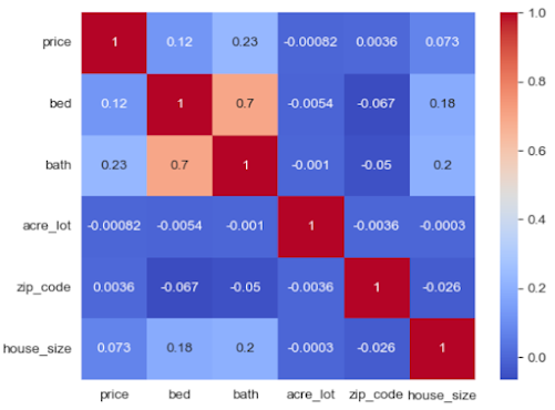
What is the correlation between house prices and other attributes? 

What could be the trend behind housing prices? 

Project: 

Step 1. Import all the packages. 

Step 4. Sort and filter the data, dropped any duplicated, Null, or NA rows, and changed the unwanted data type into the one I need. For detailed coding, please check here

Step 5. Analysis 

Find the relationship between the number of listings and states in the US 

Find the trends of prices along with the year: 

Find the relationship between Price and the number of bedrooms

Find the relationship between Price and states in the US: 

Find the correlations between price and other factor of the data: 

For detailed coding and visualization, please check my GitHub portfolio page by clicking here

Conclusion

    

            1. House prices fluctuated from 1980 to 2020, and the entire trend is going upward. 

            2. House prices are determined by many factors, such as the number of bedrooms and house size. 

            3. New York is still the top real estate market in the United States. New Jersey, Connecticut, and Massachusetts have shown higher growth than the other states. 

Thank you for watching my project. Your feedback and comments are appreciated. 

Stock Price of Top USA Banks Finance Data Project 

In this project, I used Numpy, Pandas, Seaborn, Matplotlib, Pandas_datareader  and Datetime to collect stock price data from Yahoo Finance, analyzed the data and obtain the visualization between the price and datetime of banks. Since the data was collected from Yahoo Finance, it is reliable and authenticated. However, the purpose of this project is only for study and analytics purpose, not for the realistic stock purchase purpose. The date of stock price data collected was from 1/1/2006 to 12/31/2016. 

The imports: 

Calculate the standard deviation of the returns for each bank's stock and made the plots

Plot 2008 returns for CitiGroup in 2008 only 

Imports plotply and cufflinks 

Plot all stocks for all banks during 2006 - 2016

Plot a heatmap of the correlation between the stocks close price 

Plot a clustermap for the correlations of close price

Candle plot of Bank of America's stock from 1/1/2015 to 1/1/2016 

This is the display for part of my project, including coding and visualization. If you would like to see the full picture of my project, please click here Bank Stock Python Project. 

Thank you for watching, and I would really appreciate your feedback and comment.